No Service Physical Layer issue

Technical context

Before market release, each product (telephone, UE) passes through several testing sessions, each checking various capabilities, from mechanical reliability to telecom 3GPP compliance, and more, from 3GPP specifications compliance, to data transfer performance, aging tests, etc).Telecom tests are an important part of this activity, including throughput performance, RF sensitivity, protocol compliance, power consumption, and much more.

Test description and expectations

Some of these tests are based on specific customer requirements, which need to be met even if they are not specifically mentioned by any standard (ex: 3GPP). Such an example is the ‘No Service’ test, in which the phone is kept for a long period in a no-service area (where no 2G/3G cells are available). After several hours (10..16 hours), it is removed from the shielded box, and exposed to good radio conditions.The tester will measure the time required by the telephone to find a suitable cell and camp on it.

Issue report

The issue observed was that the device under tests did not recover at all after the test, even if suitable cells were available in the area.

Physical Layer Analysis

The analysis begins at Physical Layer level, since this module is responsible with finding and synchronizing the radio cells.Info: The steps performed by the telephone, roughly, are:

1. Measurements of the surrounding cells (frequencies)
2. Sorting the results by the measured values
3. Attempting to synchronize in frequency and time the detected cells

The measurements is a simple step where frequency scanning is done, and the frequencies with higher RSSI(signal power) levels are considered potential cells.The synchronization step involves adjusting the telephone’s RF chip frequency to match the detected cell’s frequency, and then attempting to read and decode the synchronization channels of the cell. A single crystal is used by the RF chip as a reference frequency, for both 2G and 3G. For a GSM/UMTS cell to be properly detected, the RF chip has to match the cell frequency as close as possible (in the order of tens of hertz). For this it has to adjust the crystal frequency to compensate for any de-calibration (due to temperature variation, components errors, etc).During the initial synchronization phase, Layer 1 algorithms use various estimations coming from hardware modules to perform these adjustments (by changing a variable called CAFC )-  but this process still includes a lot of trial-and-error attempts.The analysis checks each synchronization step (as described above), and verifies for any inconsistencies. The first step is to verify the measurement results reported from hardware modules – to have an idea if the phone “sees” any signal or not.The verifications included the configuration of the bands to be scanned, the type of cell search algorithm (focused on speed, or on number of results), and the measurement results (RSSI values) matched with U/ARFCNs (frequencies).Using the measurement reports, a plot of the band profile is built (as seen by the telephone).

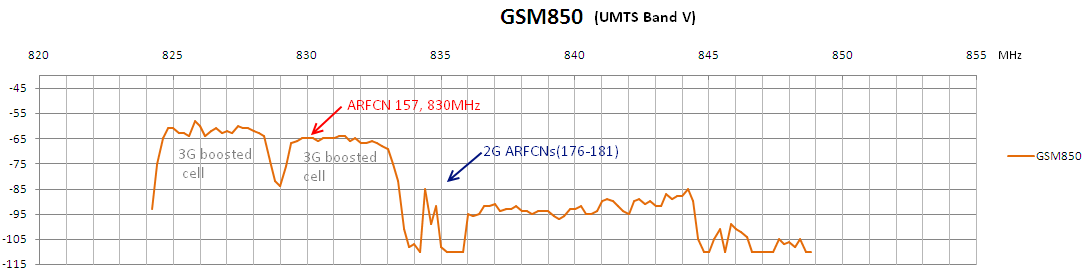
Figure 1 GSM850/UMTSV common band profileThe band profile built from the measurements matched the expected real world band profile (as observed from previous tests). This proved that the measurements algorithm worked properly.Using the band profiles, real cells can be identified by their shape and frequency width – 3G cells are 5MHz wide, while 2G cells are narrow and better separated. With this information the cell search algorithm can be matched, to confirm that the synchronization attempts are done in the right order (according to RSSI levels) and on the right frequencies (that match real cells).Supplementary, at this step, a ‚passed log’ is useful, to confirm the true cells, on which we expect the UE to synchronize.Analysis showed that synchronization attempts were done on the proper frequencies (cells) but all attempts failed when adjusting the RF crystal frequency (CAFC value), both on 2G and 3G algorithms. Even for cells with very good power levels, the frequency error estimation returned by the hardware modules returned very big values (15..20kHz), while expected values are in the range of 0 to 3kHz; this behavior was common on 2G and 3G cells – indicating a common cause. Frequency corrections with such big values usually failed – and the cell search algorithm was always interrupted at this step.Investigating the frequency estimation and correction procedures it was observed that the CAFC value (used for compensating the RF crystal frequency error) had abnormal values (ex: 6000 units), compared to the calibrated value (ex: 4200 units). This meant that each synchronization attempt began with a considerable frequency error (ex: CAFC = 6000 matched a 15kHz frequency error from the calibrated value of 4200 units).Checking the CAFC values along the cell search procedures, over a longer period of time, it was observed that sometimes the Layer 1 algorithm was not properly restoring the CAFC after a failed synchronization attempt:

1. Select an U/ARFCN to be synchronized
2. Perform an initial frequency error estimation (FCH on 2G, initial acquisition on 3G)
3. Perform the CAFC adjustment with the estimated frequency error
4. Repeat steps 2 and 3 (fine tuning)
5. If any of the adjustments fail, restore CAFC back to the initial value and try a different U/ARFCN
6. Else, continue to time synchronization (SCH on 2G) or scrambling code group detection (3G)

Sometimes, at step 5, the algorithm was restoring a different CAFC value from the starting value (step 1). For example, after two consecutive adjustments of +20kHz and +15kHz, the adjustment back (expected to be 20+15 = 35kHz) had a different value. This meant that on the next synchronization attempt, we will start with a different initial offset.On a closer look of the CAFC adjustment functions, it turned out that the intermediary frequency corrections (steps 2,3,4) were stored in a short signed int variable; each time the sum of corrections at steps 3 and 4 was bigger than +/- 32768, the variable overflowed. If synchronization failed (step 5) the algorithm was restoring back a wrong CAFC value (Figure 2).

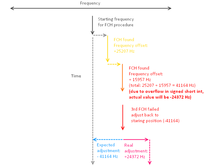
Figure 2 frequency correction accumulation and overflowIn time, these errors accumulated, leading to a significant frequency error at some point, after which the algorithm was unable to correct the frequency estimations, and no cells were synchronized anymore.

Solution

The solution was to add an overflow check, before making the frequency adjustments – because if the (total) frequency corrections are over 32kHz, that’s already an extreme (non-realistical) value.After this correction was applied, no more frequency drift accumulations occurred, and the UE was able to properly synchronize after a long time in no-service area.Many thanks to Alexandru D. for his contribution in elaborating this article. Alexandru D. is a L1 engineer within the Physical Layer team of our largest Telecom Customer Support project.